Manifolds form a collection of familiar of geometric objects encountered in the study of calculus such as, curves, surfaces, 3-dimensional regions, etc. Roughly speaking, a manifold is a subset which locally looks like Euclidian space, or Euclidian half-space.
Definition 8020
Let ![]() , X is a
manifold with boundary, of dimension k, if for every point
, X is a
manifold with boundary, of dimension k, if for every point ![]() ,there is an open subset, U, of X, such that either
,there is an open subset, U, of X, such that either
a) U is homeomorphic to ![]() ,
,
b) U is homeomorphic to Rk+ and x corresponds to a point of ![]() .
.
Remark 8026
If X is an empty set then, in a vacuous way,
it is an n-dimensional manifold for any n. As peculiar at this might first seem, it is traditional to allow this
usage.
![]()
Propositions 1.04 and 1.05, below, are important basic results. Complete proofs are beyond the scope of this text. We sketch, the proofs using Proposition 1.03.
Proposition 8032
(Invariance of domain) ![]() and
and ![]() are not
homeomorphic if
are not
homeomorphic if ![]() .
.
Proof: Assume![]() , and suppose there is a homeomorphism
, and suppose there is a homeomorphism ![]() . Let
. Let ![]() , and let
, and let ![]() and
and ![]() . Then
. Then ![]() is a homeomorphism, and thus X and Y have the same homotopy type.
is a homeomorphism, and thus X and Y have the same homotopy type.
But X has the homotopy type of Sn-1 as one can see using the deformation retraction given by:
![]()
We can use use Proposition ![]() to show that a
1-dimensional manifold cannot be homeomorphic to a two-dimensional manifold,.
In general, Proposition 1.04, the dimension of a manifold is a topological invariant:
to show that a
1-dimensional manifold cannot be homeomorphic to a two-dimensional manifold,.
In general, Proposition 1.04, the dimension of a manifold is a topological invariant:
Proposition 8059
If ![]() is a n-dimensional manifold and
is a n-dimensional manifold and ![]() is an m-dimensional manifold, if X and Y are not empty and
is an m-dimensional manifold, if X and Y are not empty and ![]() then X
and Y are not homeomorphic.
then X
and Y are not homeomorphic. ![]()
Proposition 8064
Conditions a) and b) in the above definition are
mutually exclusive. ![]()
We can use the above result to make the following two definitions.
Definition 8074
If ![]() is a manifold with boundary, then the interior of X, Int(X), is defined by
is a manifold with boundary, then the interior of X, Int(X), is defined by ![]() there is an open subset, U, of X, with U homeomorphic to
there is an open subset, U, of X, with U homeomorphic to ![]() }.
}.
Definition 8086
If ![]() is a manifold with boundary, then the boundary of X ,
is a manifold with boundary, then the boundary of X , ![]() , is defined by
, is defined by ![]() there is an open subset , U, of X, with U homeomorphic to Rk+ and x corresponds to a point of
there is an open subset , U, of X, with U homeomorphic to Rk+ and x corresponds to a point of ![]()
Remark 8093
We warn the reader not to confuse boundary of a set,
Definition 0.34, and boundary of a manifold, Definition 1.07. Similarly, we have interior of a set, Definition 0.31, and interior of a manifold, Definition 1.06. We use a capital I in ``Int'' when referring
to interior of a manifold and the lower case i in int for interior of a subset.
This is a potential source of confusion, however these are all standard
definitions. Some topologists use the term frontier of a subset to denote the boundary of the subset.
![]()
Example 8117
Consider the standard unit ball in the plane :
On the other hand, there are times when the two uses of boundary and interior do not agree. The standard inclusion of ![]() . The boundary of the set D2 and the boundary of the manifold are the same, namely the unit circle in the plane. Also the interior of the set D2 and the interior of the manifold D2 are the same, namely
. The boundary of the set D2 and the boundary of the manifold are the same, namely the unit circle in the plane. Also the interior of the set D2 and the interior of the manifold D2 are the same, namely
![]() .
So,
.
So, ![]() and int(D) = Int(D)
This example, explains why mathematicians would use the same word for two distinct concepts.
and int(D) = Int(D)
This example, explains why mathematicians would use the same word for two distinct concepts.
![]() into
into ![]() sends D2 to
sends D2 to
![]() .
The boundary of the manifold D is the circle
.
The boundary of the manifold D is the circle ![]() and the interior of the manifold D is
and the interior of the manifold D is ![]() .The interior of the set D is the empty set and the boundary of the set D is all of D, so in this case
.The interior of the set D is the empty set and the boundary of the set D is all of D, so in this case ![]() and
and ![]() .
. ![]()
Example 8120
Any interval in ![]() (open, closed, half-open) is a
1-dimensional manifold.
(open, closed, half-open) is a
1-dimensional manifold.
Example 8130
For each k, Sk is a k-dimensional manifold. Also ![]() is a k-dimensional manifold, as well as any open subset of
is a k-dimensional manifold, as well as any open subset of ![]() All these examples have empty boundary.
All these examples have empty boundary. ![]()
Example 8138
Example 8152
Use polar coordinates, and let
Using spherical coordinates, we could let ![]() ,
, ![]() . This 2-dimensional manifold is an annulus, see Definition
. This 2-dimensional manifold is an annulus, see Definition ![]() . Here
. Here ![]() consists of two disjoint circles:
consists of two disjoint circles: ![]() , and
, and ![]() .
.![]() . This is a 3-dimensional manifold and
. This is a 3-dimensional manifold and ![]() is the disjoint union of two concentric spheres:
is the disjoint union of two concentric spheres: ![]() , and
, and ![]() .
. ![]()
Using Proposition 1.05 one can show:
Proposition 8160
If X is an n-dimensional manifold, then int(X) is
an n-dimensional manifold, and ![]() is an (n-1)-dimensional
manifold (possibly empty).
width4pt height6pt depth1.5pt
is an (n-1)-dimensional
manifold (possibly empty).
width4pt height6pt depth1.5pt
Consider that ![]() is a circle, and the circle has empty boundary. Similarly,
is a circle, and the circle has empty boundary. Similarly, ![]() is a sphere, and the boundary of this sphere is the empty set. In general
we have the following.
is a sphere, and the boundary of this sphere is the empty set. In general
we have the following.
Proposition 8166
If X is a manifold, then ![]() .
width4pt height6pt depth1.5pt
.
width4pt height6pt depth1.5pt
Proposition 8170
If ![]() is an n-manifold, it is locally connected.
is an n-manifold, it is locally connected.
Remark 8174
Proposition 1.16 implies that the topologist's ![]() curve is not a manifold.)
curve is not a manifold.)
![]()
Here is a basic question about manifolds:
Question 8178
a given natural number, n, how many n-dimensional manifolds are there? By this we mean--how many homeomorphism classes of such manifolds are there? Are there uncountably many homeomorphism classes of manifolds ?
Remark 8184
One-dimensional manifolds are familiar subsets.
An example of a compact, disconnected one dimensional manifold is a union of
two disjoint circles. By considering unions of more and more circles, one sees that there are infinitely many one-dimensional manifolds, no two of which are homeomorphic.
An example of a connected one-dimensional manifold
which is not compact is ![]() . An example of a compact, connected
one-dimensional manifold with non-empty boundary is I.
. An example of a compact, connected
one-dimensional manifold with non-empty boundary is I.
![]()
Proposition 8189
If X is a connected, compact, one-dimensional manifold
with empty boundary, then X is homeomorphic to a circle.
![]()
One of the goals in topology is to capture the nature of certain subsets terms of topological properties.
Proposition 1.20 is a statement of this sort. But we cannot extend this result to the two dimensional sphere easily since there are compact, connected, two-dimensional manifolds which are not homeomorphic to S2. One example of this is the torus, see Definition 1.22.
 |
 |
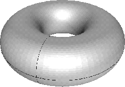
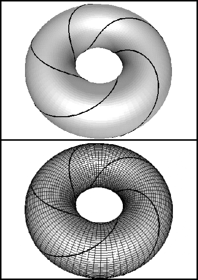
Example 8235
The torus is an important 2-dimensional manifold, see Figure 1-1. We describe it as a subset of
For any angle,
You may think of the letter ``D'' of D(a,b), here as referring to ``donut''; the circles
The torus is the image of a continuous
map that will play an important role in later Chapters.
Let a and b be numbers with 0 < a < b . Define a function,
No particular choice of a and b is mathematically special,
but for the sake of being specific we chose to focus on T(1,2).
![]() .Informally, we an speak of the torus as the ``surface of a donut'', D(a,b), where the
``thickness of the donut" is 2b and ``size of the hole'' is 2(a - b).
Of course we need b<a.
We may describe a torus as a surface obtained ``by spinning a
circle about about the z-axis''. Let C be the circle in the x-y-plane
with center at the origin and radius a. The circle C will correspond to the ``core circle or the donut''.
Using cylindrical coordinates, we describe C as all points
.Informally, we an speak of the torus as the ``surface of a donut'', D(a,b), where the
``thickness of the donut" is 2b and ``size of the hole'' is 2(a - b).
Of course we need b<a.
We may describe a torus as a surface obtained ``by spinning a
circle about about the z-axis''. Let C be the circle in the x-y-plane
with center at the origin and radius a. The circle C will correspond to the ``core circle or the donut''.
Using cylindrical coordinates, we describe C as all points ![]() with r=a, z=0.
with r=a, z=0.
![]() consider the page
consider the page ![]() (recall Definition 0.13). In cylindrical coordinates, let
(recall Definition 0.13). In cylindrical coordinates, let ![]() be the circle in
be the circle in ![]() with center
with center ![]() and radius b, and let
and radius b, and let ![]() be the closed disk in
be the closed disk in ![]() with the same center and radius.
Let
with the same center and radius.
Let ![]() , and
, and ![]() .
.![]() , will later be referred to as ``meridians''.
, will later be referred to as ``meridians''.
![]() , (using Cartesian coordinates, this time) by
, (using Cartesian coordinates, this time) by
![]()
![]()
Definition 8246
The standard torus T2, in ![]() is defined to
be T(1,2). The standard covering map
is defined to
be T(1,2). The standard covering map ![]() is
the map described above with a = 2 and b = 1.
is
the map described above with a = 2 and b = 1.
The set D(2,1) is called the standard solid torus in ![]() . The circle C is called the core of the standard solid torus.
. The circle C is called the core of the standard solid torus.
Later, we will examine the torus as a subset of
![]() , Definition
, Definition ![]() .
.
 |
 |
 |
 |
 |
Example 8271
us examine, in detail, the map P.
Certainly P is not a one-to-one function.
In fact if p and q are integers
then ![]() .
More
generally, for any real numbers x and y and integers p and q, we
have
.
More
generally, for any real numbers x and y and integers p and q, we
have ![]() . Thus every point
of T(a,b) is the image of infinitely many points, see Figure 1-2. Note however that P
is one-to-one on the subset
. Thus every point
of T(a,b) is the image of infinitely many points, see Figure 1-2. Note however that P
is one-to-one on the subset ![]() .
. ![]()
Example 8295
We can use the map P to describe
interesting subsets of the torus. Suppose that l(A,B,C) is
the line in the plane with equation A x + B y = C (with A and B not
both zero). Then we can define L(A,B,C) = P(l(A,B,C)).
The sets L(1,0,0) and L(0,1,0)
are circles on the torus. Generally, any of the circles L(1,0,C) are called a longitude of the torus,
a circle L(0,1,C) is call a meridian of the torus,
see Figure 1-1
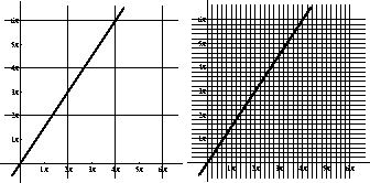
In our figures, we can visually verify the type of curve using a grid for the plane.
When we transfer this the image of such a grid to the torus, using P we get a curvilinear grid. For example the line and grid shown in Figure 1-3 transfers to the circle and circular grid as shown in the bottom figure of Figure 1-4. A similar example is shown in the pair Figure 1-5 and Figure 1-4
For any two rational numbers, r and q,
L(r,q,0) is homeomorphic to a circle.
Such a set can be described as
``the image, under P, of a line in the plane through the origin with
rational slope''.
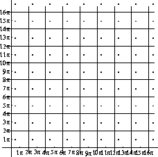
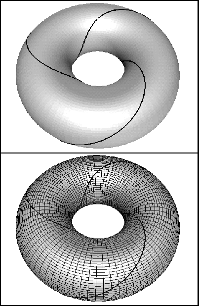
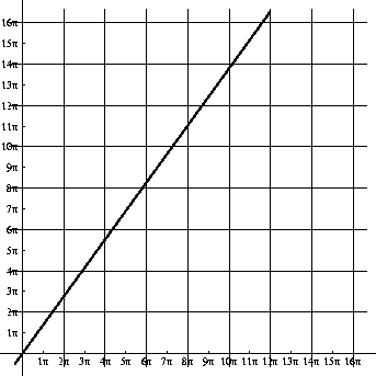
In Figure 1-4 we see the curve l(3,-2,0). Here, of course L(3,-2,0) is a line with slope 3/2 thus traverses 3 squares in the y-direction for every two squares in the x-direction , see Figure 1-3. On the torus we can visually verify the type of curve by noting that it traverses the curvilinear grid three units in a meridian direction for every two in the longitude direction, Figure 1-4.
Similarly one has the curve l(5,-3,0), see Figures 1-5 and 1-6.
![]()
 |
 |
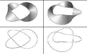 |
Example 8351
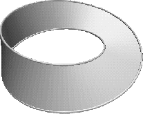
We describe an interesting subset of
Consider the circle L(2,-1,0), in
We will call M the standard Möbius band in
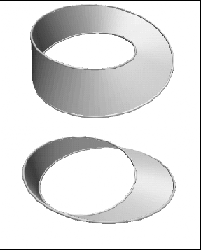
We could similarly consider the circle L(2,1,0). This also meets each
Clearly, M and
Of course one can get other Möbius bands with other curves. In Figure 1-10 we show Möbius bands constructed using the circles L(3,-1,0) and L(3,1,0).
The fact that the Möbius bands of Figure 1-9 and Figure 1-10 look so different is a reflection of the fact (which we do not prove) that these are not equivalent subsets of ![]() , the Möbius band. A rough description of this is: a band with a half twist.
The Möbius band in
, the Möbius band. A rough description of this is: a band with a half twist.
The Möbius band in ![]() will be described as a union of line segments whose endpoints lie on a circle.
will be described as a union of line segments whose endpoints lie on a circle.
![]() . Clearly each page,
. Clearly each page, ![]() , of
, of ![]() intersects L(2,-1,0) in exactly two points. For any
intersects L(2,-1,0) in exactly two points. For any ![]() , let
, let ![]() be the line segment in
be the line segment in ![]() with those two points as endpoints. (We note that
with those two points as endpoints. (We note that ![]() .).
Define:
.).
Define: ![]() , see Figure 1-8.
, see Figure 1-8.
![]() .
Generally, any subset homeomorphic to the standard Möbius band will be called a Möbius band. We will call M the standard Möbius band in
.
Generally, any subset homeomorphic to the standard Möbius band will be called a Möbius band. We will call M the standard Möbius band in ![]() .
It is clear from the Figure 1-8 that M is a 2-dimensional manifold and
.
It is clear from the Figure 1-8 that M is a 2-dimensional manifold and ![]() .
.![]() in two points. For any
in two points. For any ![]() , let
, let ![]() be the line segment in
be the line segment in ![]() between these points. We let
between these points. We let ![]() be the union of these line segments:
be the union of these line segments: ![]() , see Figure 1-9.
, see Figure 1-9.
![]() are homeomorphic, in fact, by a homeomorphism that takes
are homeomorphic, in fact, by a homeomorphism that takes ![]() to
to ![]() .
We can describe
.
We can describe ![]() also as a band with a half twist, but this half twist is in the opposite direction as if seen in a mirror.
Consider,
also as a band with a half twist, but this half twist is in the opposite direction as if seen in a mirror.
Consider, ![]() defined by m(x,y,z) = (x, y -z). We can see m is a homeomorphism, in fact, a rigid motion, of
defined by m(x,y,z) = (x, y -z). We can see m is a homeomorphism, in fact, a rigid motion, of ![]() which takes M to
which takes M to ![]() . Sometimes m is described as a mirror reflection in the x-y-pane.
We call
. Sometimes m is described as a mirror reflection in the x-y-pane.
We call ![]() the mirror image of M.
the mirror image of M.
![]() .
.![]()
Example 8392
One gets interesting subsets of the torus by taking lines
with irrational slopes.
Consider a line l = m x, with irrational slope; let L = P(l).
Claim: that L is dense in T2, see Definition 0.06 for definition of dense.
As an example, we focus at one point, Z = (3,0,0) of T2, and leave as an exercise proof for an arbitrary point of T2.
Let U be an open subset of T2 containing Z, we want to find a point of L in U.
Using P, We transfer this problem to a problem in the plane. Let
For any integer, N, the line l intersects the vertical line
Not only is L a dense subset of T2, it has some other interesting properties. Further analysis shows
that L fails to be locally connected at every point! In particular this shows that
L is not a manifold, even though it is the image of a manifold and P|l is an immersion. ![]() ;
; ![]() .In Figure 1-7, we show the line L;
.In Figure 1-7, we show the line L; ![]() corresponds to the grid points.
We need to show we can find points of l arbitrarily close to a grid point.
corresponds to the grid points.
We need to show we can find points of l arbitrarily close to a grid point.
![]() at
at ![]() . Since m is irrational,
. Since m is irrational, ![]() is an irrational multiple of
is an irrational multiple of ![]() . So we need to show that, given
. So we need to show that, given ![]() , we can find an N so that, for some Q, the distance from
, we can find an N so that, for some Q, the distance from ![]() and
and ![]() is less than
is less than ![]() .This follows from the proof of Example 0.41. There we showed we can find
multiples of angle
.This follows from the proof of Example 0.41. There we showed we can find
multiples of angle ![]() arbitrarily close to a multiple of
arbitrarily close to a multiple of ![]() .
.![]()
Example 8422
We give an alternate description of the torus and solid torus and some related manifolds.
The standard solid torus, D(2,1), in
We can describe the torus using the idea of distance from a point to a set.
Let C the circle as in Example 1.21--centered at the origin, in the x-y-coordinate plane, of radius 2.
Then T2 consists of those points in
Let
Also
Our final example is, W, consists of a ball of radius 4 with the interior of the standard solid torus removed.
If we let ![]() is a 3-dimensional manifold whose boundary is the standard torus, T2 see Definition 1.22.
is a 3-dimensional manifold whose boundary is the standard torus, T2 see Definition 1.22.
![]() whose distance to C is 1; D(2,1) consists of those points whose distance to C is greater than or equal to 1.
More formally, consider the map
whose distance to C is 1; D(2,1) consists of those points whose distance to C is greater than or equal to 1.
More formally, consider the map ![]() defined by
defined by ![]() . Then f-1 (1) = T2.
. Then f-1 (1) = T2.
![]() ,
, ![]() . It is not hard to show that both U and V are connected. In fact, they are path connected.
It follows then that
. It is not hard to show that both U and V are connected. In fact, they are path connected.
It follows then that
![]() has two components: V, which is
bounded and U, which is unbounded.
has two components: V, which is
bounded and U, which is unbounded.
![]() is an interesting
non-compact 3-dimensional manifold whose boundary is a torus.
is an interesting
non-compact 3-dimensional manifold whose boundary is a torus.
![]() , then W is a compact 3-dimensional manifold whose boundary has two components--one of which is homeomorphic to a sphere and the other to a torus.
, then W is a compact 3-dimensional manifold whose boundary has two components--one of which is homeomorphic to a sphere and the other to a torus.
![]()
 |
 |
Example 8440
We say that the torus has a hole (thinking of the ``hole in
the donut").
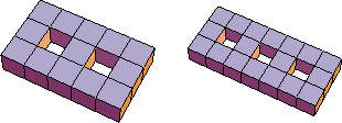
Some other examples of manifolds of dimensions 2 and 3 are variations of the torus and solid torus ``with several holes''.
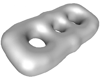
Picture two- and three- holed ``bricks'' as in Figure 1-11. Considered topologically, these are called the solid 2-holed torus and the solid 3-holed torus, respectively. The surfaces of these bricks are called the 2-holed torus and 3-holed torus respectively. A more traditional, smoother version of a 3-holed torus is shown in Figure 1-12
More generally we can have an n-holed torus.
In contrast to the torus, it is not easy (nor profitable for us) to describe these examples
with equations. ![]()
Question 8444
is a mathematical definition of ``hole" as used above?
That is, is there a topological property ``the number of holes of X'' so
that the torus has one hole, etc? ![]()
The answer to the above question is the beginning of the subject of algebraic topology and is beyond the scope of this book.
At this point it is handy to introduce a definition:
Definition 8448
If ![]() is a manifold which is compact with empty boundary, then we say that the manifold M is closed.
is a manifold which is compact with empty boundary, then we say that the manifold M is closed.
Remark 8460
Once again we see that words are used for manifolds which do not have the same meaning as for subsets.
If M is a closed manifold and ![]() , then M is also a closed subset of X, since all compact subsets are closed subsets.
The closed n-ball Dn, 0 < n, is a compact subset of
, then M is also a closed subset of X, since all compact subsets are closed subsets.
The closed n-ball Dn, 0 < n, is a compact subset of ![]() which is not a closed manifold, since
which is not a closed manifold, since ![]() .
. ![]()
There are other similarities between the notion of boundary of a set and boundary of a manifold. Compare the result below to similar statements about the boundary of a set: Proposition 0.37 c), also consult Remark 0.39 and Figure 0-7.
Proposition 8474
Suppose that M is an m-manifold and N is an n-manifold. Then ![]() .
.
Let ![]() and
and ![]() . Then
. Then ![]() is an (n+m)-manifold,
and
is an (n+m)-manifold,
and ![]() is the union of A and B . Furthermore,
is the union of A and B . Furthermore, ![]() .
width4pt height6pt depth1.5pt
.
width4pt height6pt depth1.5pt
The proof of the above is not too difficult if either ![]() or
or ![]() .
.
We can obtain bountiful supply of manifolds (generally non-compact) by using the next proposition.
Proposition 8484
If X is an n-dimensional manifold and C is a closed subset of int(X), then X - C is an n-dimensional manifold. width4pt height6pt depth1.5pt
Remark 8496
In particular, any open subset of
Suppose K is a subset of ![]() is an n-dimensional
manifold. Also, if we remove a finite number of points from an n-holed
torus, we get a two-dimensional manifold.
is an n-dimensional
manifold. Also, if we remove a finite number of points from an n-holed
torus, we get a two-dimensional manifold.
![]() such that K is homeomorphic to S1. Examples where K is ``knotted" give rise to interesting
three-dimensional manifolds by considering
such that K is homeomorphic to S1. Examples where K is ``knotted" give rise to interesting
three-dimensional manifolds by considering ![]() . This will be discussed in more detail in Chapter
. This will be discussed in more detail in Chapter ![]() .
.
![]()
Proposition 8501
Suppose ![]() is a connected k-dimensional manifold, then M is path connected.
is a connected k-dimensional manifold, then M is path connected.
Proof: Let ![]() . Let U be the set of points, q, of M, such that there is a path, in M, from p to q. Let V be the set of points, q, of M that there is no path in M from p to q. Our goal is to show that
. Let U be the set of points, q, of M, such that there is a path, in M, from p to q. Let V be the set of points, q, of M that there is no path in M from p to q. Our goal is to show that ![]() .
.
Certainly, ![]() since
since ![]() .
We next show that U is an open subset of M. Suppose
.
We next show that U is an open subset of M. Suppose ![]() ; then there is a path
; then there is a path ![]() from p to x. Since M is a manifold, there is an open subset, W, of M, with
from p to x. Since M is a manifold, there is an open subset, W, of M, with ![]() such that W is either homeomorphic to
such that W is either homeomorphic to ![]() or Rk+; call this homeomorphism h.
Let
or Rk+; call this homeomorphism h.
Let ![]() . Since
. Since ![]() and Rk+ are path connected, we can find a path
and Rk+ are path connected, we can find a path ![]() from h(x) to h(y).
Let
from h(x) to h(y).
Let ![]() , then
, then ![]() is a path in W from x to y. Finally
is a path in W from x to y. Finally ![]() is a path from p to y, where * denotes concatenation of paths, recall Definition 0.40. Thus U is an open subset of M since, for every point of U, there is an open subset, W, of M, which is contained in U.
is a path from p to y, where * denotes concatenation of paths, recall Definition 0.40. Thus U is an open subset of M since, for every point of U, there is an open subset, W, of M, which is contained in U.
A variation of the above argument shows that V is open. Suppose ![]() ; we can find a W, open in M, homeomorphic to
; we can find a W, open in M, homeomorphic to ![]() or Rk+. Since any point of W can be joined to x be a path in W, it follows that no point of W can be joined by a path in M to p. This means that V is an open subset of M.
or Rk+. Since any point of W can be joined to x be a path in W, it follows that no point of W can be joined by a path in M to p. This means that V is an open subset of M.
We conclude that V must be an empty subset since, otherwise, U and V would form a disconnecting partition of M contradicting the assumption that M is connected. width4pt height6pt depth1.5pt
Remark 8580
Proposition 1.05 basically says that, topologically, boundary points do not look like interior points. In particular, this means that a manifold with non-empty boundary cannot be homogeneous.
However the next Proposition states that a connected manifold with empty boundary is homogeneous.
One needs the connectedness hypothesis if the manifold has components which are not homeomorphic. We will later prove that a sphere and a torus are not homeomorphic. If X is a subset with two components, S and T with S homeomorphic to the sphere and T homeomorphic to a torus, then X cannot be homogeneous since a homeomorphism must take a component to a component.
![]()
Proposition 8587
Suppose ![]() and M is a connected manifold with
and M is a connected manifold with ![]() , then M is homogeneous.
, then M is homogeneous. ![]()
Remark 8637
The proof of Proposition 1.37 is difficult and depends on basic results too technical to prove here. However we can give a sketch of a proof. Suppose x and y are points of M.
The idea is to find an open subset, U, of M homeomorphic to
Using h we obtain another homeomorphism,
Here is the idea of how to find U. By Proposition 1.35 we know that there is a path, ![]() which contains x and y, this is the ``hard part'' of the proof. Suppose we had such a homeomorphism, h.
From this point it is not difficult to finish. The idea is to use homogeneity of
which contains x and y, this is the ``hard part'' of the proof. Suppose we had such a homeomorphism, h.
From this point it is not difficult to finish. The idea is to use homogeneity of ![]() move x to y inside U, while keeping things fixed outside of U.
move x to y inside U, while keeping things fixed outside of U.
![]() so that
so that ![]() and
and ![]() are contained in the standard open unit ball in
are contained in the standard open unit ball in ![]() .We know that
.We know that ![]() is homogeneous. Moreover, one can find a homeomorphism,
is homogeneous. Moreover, one can find a homeomorphism, ![]() such that
such that ![]() and
and ![]() .Define
.Define ![]() by
by
![]()
![]() from x to y,
from x to y, ![]() . With a non-trivial amount of work we can improve this to show that, in fact there is a path from
. With a non-trivial amount of work we can improve this to show that, in fact there is a path from ![]() from x to y such that
from x to y such that ![]() is an embedding. We then obtain U as a ``thin'' open subset containing
is an embedding. We then obtain U as a ``thin'' open subset containing ![]() --we chose a small
--we chose a small ![]() and then U is the set of points if M a distance less than
and then U is the set of points if M a distance less than ![]() from a point of
from a point of ![]() , The next step is to show that for a small enough choice of
, The next step is to show that for a small enough choice of ![]() , this subset is homeomorphic to
, this subset is homeomorphic to ![]() .
. ![]()
 |
 |
 |
 |
As noted in Remark 1.36, a manifold M with non-empty boundary is not homogeneous, but we can obtain a version of homogeneity by treating ![]() specially.
specially.
In Proposition 1.40, we prove a special case of Proposition 1.39, below. We will use the particular special case in a discussion in
in Chapter ![]() .
.
Proposition 8685
Suppose ![]() and M is a compact connected manifold with
and M is a compact connected manifold with ![]() , and if p and q are points of Int(M), then there is a homeomorphism, h, of M onto M such that h(p) = q and
, and if p and q are points of Int(M), then there is a homeomorphism, h, of M onto M such that h(p) = q and ![]() .
. ![]()
Proposition 8696
Suppose D2 and be standard unit ball. If p and q are points of Int(D2), then there is a homeomorphism, h, of D2 such that h(p) = q and ![]() .
.
Proof:
First we investigate a ``lower dimensional'' version of our problem: given two points of Int(D1) is there a homeomorphism fixed on ![]() that takes one point to the other? Since D1 is a closed interval [-1,1], and
that takes one point to the other? Since D1 is a closed interval [-1,1], and ![]() is the two point set
is the two point set ![]() , this is not hard to do. We then apply this result to obtain a map of a square to itself, considering one coordinate at a time.
, this is not hard to do. We then apply this result to obtain a map of a square to itself, considering one coordinate at a time.
This map is not quite we want. It sends the boundary of the square to itself, but is not the identity map there. The next step is to improve this by changing the map near the boundary of the square. Finally, since the square is homeomorphic to D2, we ``transfer'' this to a map to the square to itself to a map of D2 to itself.
Now for the details.
Let h be a homeomorphism: ![]() , and let
, and let
![]() . Write coordinates of these points as:
. Write coordinates of these points as: ![]() . Define
. Define ![]() to be the piecewise linear function such that
to be the piecewise linear function such that ![]() . Also define
. Also define ![]() to be the piecewise linear function such that
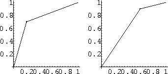
to be the piecewise linear function such that ![]() , see Figure 1-14. (Note: f and g are solutions of a corresponding 1-dimensional problem.) Define a map
, see Figure 1-14. (Note: f and g are solutions of a corresponding 1-dimensional problem.) Define a map ![]() by
G(x,y) = (f(x), g(y)). Since f and g are homeomorphisms, G is a homeomorphism with, G(P) = Q.
by
G(x,y) = (f(x), g(y)). Since f and g are homeomorphisms, G is a homeomorphism with, G(P) = Q.
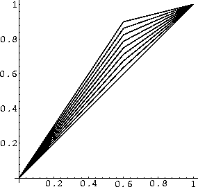
We can check that ![]() , but, as can be seen in Figure 1-15,
, but, as can be seen in Figure 1-15, ![]() .
.
We find a sub-square, X, of ![]() which contains P and Q. Our idea is to use the map we have on this sub-square, and define a different map on
which contains P and Q. Our idea is to use the map we have on this sub-square, and define a different map on ![]() . That is, we find a homeomorphism
. That is, we find a homeomorphism ![]() , such that
, such that ![]() , and
, and ![]() .
Figure 1-16 gives the idea of how this is to be done.
.
Figure 1-16 gives the idea of how this is to be done.
Further details shed little further light on the matter. But, as a concrete example of how one constructs such a homeomorphism, here are some of those details.
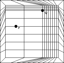
Let ![]() , and let
, and let
![]() . We have P and Q points of X.
. We have P and Q points of X.
For any ![]() ,
, ![]() maps the interval
maps the interval ![]() to itself by moving the point (x,y) to the point (x,g(y)) but on
to itself by moving the point (x,y) to the point (x,g(y)) but on ![]() we want (0,y) to go to (0,y). In other words, looking at vertical line segments, we want a map ``changes from g to the identity map'' as x gets close to zero. Looking at Figure 1-15
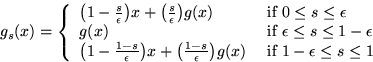
we get an idea of what we want to do. A standard way to get a family of functions that change from the identity to g is to consider (1-s) x + s g(x); If s=0 then this function is x, if s=1 it is g(x).
We want to arrange it so that for
we want (0,y) to go to (0,y). In other words, looking at vertical line segments, we want a map ``changes from g to the identity map'' as x gets close to zero. Looking at Figure 1-15
we get an idea of what we want to do. A standard way to get a family of functions that change from the identity to g is to consider (1-s) x + s g(x); If s=0 then this function is x, if s=1 it is g(x).
We want to arrange it so that for ![]() , the map we get is g(x).
For
, the map we get is g(x).
For ![]() , let
, let ![]() . Then g0 (x) = x and
. Then g0 (x) = x and ![]() .
.
Consider the other three sides of ![]() . Completing the above analysis, we end up with the following definitions:
. Completing the above analysis, we end up with the following definitions:
and
Now define ![]() . For any y, fy is a homeomorphism (it is a monotone increasing function, since it is a linear combination of monotone increasing functions). From this we conclude that
. For any y, fy is a homeomorphism (it is a monotone increasing function, since it is a linear combination of monotone increasing functions). From this we conclude that ![]() is 1-to-1 and onto. Since each of the coordinate functions is continuous, it follows that
is 1-to-1 and onto. Since each of the coordinate functions is continuous, it follows that ![]() is continuous. Since
is continuous. Since ![]() is compact, we conclude that
is compact, we conclude that ![]() is a homeomorphism. Since we have explicit formulas, we can check that
is a homeomorphism. Since we have explicit formulas, we can check that ![]() , and
, and ![]() .
.
As a final step we transfer this function to a homeomorphism of D2 by conjugation by h. Let ![]() , then H is a homeomorphism of D2, fixed on
, then H is a homeomorphism of D2, fixed on ![]() such that H(p) = q.
such that H(p) = q.
width4pt height6pt depth1.5pt
Historically, the interest in the topic of manifold, arose from analysis. There
focus is on subsets of ![]() for which we can apply the basic concepts of calculus such as: tangent lines to curves, and tangent planes for surfaces.
A differentiable function, is continuous, but there are continuous functions such as f(x) = |x| which are continuous but not differentiable.
for which we can apply the basic concepts of calculus such as: tangent lines to curves, and tangent planes for surfaces.
A differentiable function, is continuous, but there are continuous functions such as f(x) = |x| which are continuous but not differentiable.
A smooth function is a differentiable function, in fact generally in topology one assumes that the functions involved are (infinitely) differentiable. For most purposes, the hypothesis that functions have continuous second derivatives is all that is required. So assuming higher derivatives is more convenience than necessity. Most definitions of derivative require an open domain so the definition below is in two parts, one for open subsets, a second for arbitrary subsets.
Definition 8795
Suppose U is an open subset of ![]() and
and ![]() is a function written as
is a function written as
![]()
If ![]() and
and ![]() , we say f is smooth if there is an open subset U of
, we say f is smooth if there is an open subset U of ![]() , and a smooth map
, and a smooth map ![]() , such that F|X = f and F is smooth.
, such that F|X = f and F is smooth.
Definition 8804
Suppose ![]() ,
, ![]() and
and ![]() is a homeomorphism. If f is also smooth then we say F is a diffeomorphism. If a diffeomorphism exists, then we say that X and Y are diffeomorphic.
is a homeomorphism. If f is also smooth then we say F is a diffeomorphism. If a diffeomorphism exists, then we say that X and Y are diffeomorphic.
Definition 8820
Let ![]() , X is a smooth
manifold with boundary, of dimension k, if for every point
, X is a smooth
manifold with boundary, of dimension k, if for every point ![]() ,there is an open subset, U, of X such that either
,there is an open subset, U, of X such that either
a) U is diffeomorphic to ![]() ,
,
b) U is diffeomorphic to Rk+ and x corresponds to a point of ![]() .
.
Example 8835
![]() is and Rn+ are smooth manifolds, for any n. Similarly any open subset of
is and Rn+ are smooth manifolds, for any n. Similarly any open subset of ![]() or Rn+ is a smooth manifold.
or Rn+ is a smooth manifold.
To show that Sn is a smooth manifold is not hard. We can use stereographic projection, see Proposition 0.20, to get a smooth map from ![]() where
where ![]() is the ``south pole'',.
Then we use a similar map for
is the ``south pole'',.
Then we use a similar map for ![]() where
where ![]() is the ``north pole'',
is the ``north pole'', ![]() .
.
![]()
The following idea is is a familiar one from calculus. A regular value is a value which is not the image of any critical point.
Definition 8844
Suppose ![]() is a smooth function is
is a smooth function is ![]() . We say that y is a regular value
of f if for all points,
. We say that y is a regular value
of f if for all points, ![]() , some partial derivative,
, some partial derivative, ![]() .
.
With the next Proposition, we can find many smooth manifolds.
Proposition 8852
Suppose ![]() is a smooth function is
is a smooth function is ![]() and y is a regular value for f. Then f-1 (y) is a smooth (n-1)-dimensional manifold with empty boundary.
and y is a regular value for f. Then f-1 (y) is a smooth (n-1)-dimensional manifold with empty boundary.
Remark 8857
Manifolds obtained by the Proposition 1.46, are familiar constructions. For maps of ![]() , these are the level curves; for
, these are the level curves; for ![]() these are level surfaces.
these are level surfaces.
![]()
A smooth manifolds is sometimes called a differentiable manifold . The study of smooth manifolds is called differential topology.
To go much further into this topic would entail a whole book (such as [GP,HR2]), but at least we can state one basic problem.
Question 8861
X and Y are homeomorphic smooth manifolds are they diffeomorphic?
Remark 8872
The answer to this question is ``no''! This is a long and interesting story, we mention only a few of the highlights. Basically, in low dimensions, there is not much problem. But there are smooth 7-dimensional manifolds that are homeomorphic to S7 but not diffeomorphic to S7. As a matter of fact, there are exactly 27 different (mutually non-diffeomorphic) such examples.
As a rule, in topology, a situation is simpler in the compact case compared to the non-compact case.
The case Question of 1.48 for, ![]() , is a notable exception to this rule: if X is homeomorphic to
, is a notable exception to this rule: if X is homeomorphic to ![]() , then it is diffeomorphic to
, then it is diffeomorphic to ![]() , except for
, except for ![]() , in which case there are infinitely many non-diffeomorphic examples.
, in which case there are infinitely many non-diffeomorphic examples.
![]()
PROBLEMS FOR CHAPTER ![]()
Problem 8875
that an n-dimensional manifold has dimension n, according to Definition ![]() .
.
Problem 8880
that if X is a two-dimensional manifold and if Y is a one dimensional manifold that X and Y are not homeomorphic.
Problem 8885
that
D2 is a 2-dimensional manifold and ![]() . ( Hint: for points of S1 you might consider the complex exponential map. )
. ( Hint: for points of S1 you might consider the complex exponential map. )
Problem 8888
Proposition 1.32 in the case that if either ![]() or
or ![]() .
.
Problem 8889
Proposition 1.16.
Problem 8894
M be a k-dimensional manifold. Show that each component of M is a k-dimensional manifold.
Problem 8902
![]() and M is a k-dimensional manifold.
Show that
and M is a k-dimensional manifold.
Show that ![]() . (Note: be careful to distinguish int and Int.) Also show that
. (Note: be careful to distinguish int and Int.) Also show that ![]() .
.
Problem 8908
that if M is a connected k-manifold with 1 <k and ![]() then
then ![]() is a connected set.
is a connected set.
Problem 8909
that the standard torus does not have the fixed point property.
Problem 8913
the statement of Remark 1.24 that for any two rational numbers, r and q that L(r,q,0) is a circle.
Problem 8915
the proof in Exercise 1.26 for an arbitrary point of T2.
Problem 8919
that T2 - L and L fail to be locally connected at every point, where L is as in Example 1.26.
Problem 8922
that the subsets U and V of Example 1.27are path connected.
Problem 8926
that for the subsets defined in Example 1.27, that ![]() and also that
V = int(D(2,1)) = Int(D(2,1) and
and also that
V = int(D(2,1)) = Int(D(2,1) and ![]() .
.
Problem 8927
the details of the claims of the middle paragraph of Remark 1.38.
Problem 8930
formulas for the piecewise functions f and g as described in the proof of Proposition 1.40.
Problem 8933
, directly, that for any n, Sn is homogeneous.
Problem 8937
, directly, that the torus , T2 is homogeneous. (Hint: use the map ![]() and the homogeneity of
and the homogeneity of ![]() ).
).
Problem 8939
that the circle, S2 is a smooth manifold, see Example 1.44.